Quantum Holistic Theory
Holistic Approach: Bridging Quantum Mechanics and Reality
Top Position in Science - The 90.10.-CUBE (2022/07)
Introduction to Quantum Holistic Theory
The Holistic Theory integrates the principles of quantum mechanics and general relativity, proposing a comprehensive and unified understanding of the universe.
This model accentuates:
Physical and Psychological Health: Mirroring the vastness of cosmic scales and the curvature of spacetime, while also recognizing the intricate interplay of our mental and physical well-being.
Intellectual & Consciousness Health: This underscores the all-encompassing perspective where quantum particles’ intricate behaviors are interwoven. Within this structure, both Intellect and Consciousness act as foundational pillars, grounding the Universe’s Information and Quantum Information Fields. This Quantum Holistic Theory lays the intellectual groundwork for Homo Quanticum Centrism.
Neuronal & Emotional Health: This underscores the crucial role of the observer, suggesting that an individual’s consciousness and emotions might play a significant role in shaping reality.
Science and Spiritual Health: Identifies with the core of Quantum Centrism, revealing the symbiosis between Quantum Technology and Quantum Biology, and bridging the divide between scientific inquiry and spiritual understanding, paving the way to a deeper understanding of Intellectual and Emotional Consciousness.
It presents a comprehensive perspective on reality, underscoring the symbiotic relationship between Physical, Psychological, Intellectual, Neuronal, Spiritual, and Scientific health, all under the umbrella of Homo Quanticum Centrism.
The Rindler horizon delineates a boundary in spacetime, demarcating areas accessible to a perpetually accelerating observer from regions perpetually elusive. While akin to a black hole’s event horizon, it does not pertain to spacetime curvature, but rather stems from the effects of special relativity. This concept is attributed to Wolfgang Rindler, who delved into the intricacies of uniformly accelerating frames within a flat spacetime [1].
Conversely, the Heisenberg uncertainty principle is a cornerstone of quantum mechanics. It postulates that precise simultaneous measurements of a particle’s position and momentum are inherently limited. The more exact the position’s measurement, the more indeterminate the momentum becomes, and vice versa. This principle assures that the uncertainties’ product in position and momentum always surpasses a particular constant, closely tied to Planck’s constant. Similar principles hold for other conjugate variable pairs, like energy-time or frequency-time [2].
[1] Wikipedia: Rindler coordinates
[2] Greg Egan, “The Rindler Horizon“
While the Rindler horizon and the Heisenberg uncertainty principle derive from distinct physics realms, intriguing scenarios might intertwine both concepts. Picture an observer in a constantly accelerating spaceship, distancing from a consistent-frequency photon source. Due to the Doppler effect, observed photons from the source will exhibit redshift, with decreasing frequency as they near the Rindler horizon. When trying to ascertain the photon’s position and frequency, the observer encounters the Heisenberg constraint: ΔxΔf ≥ c/4π. Consequently, as frequency uncertainty lessens, position ambiguity swells, and vice versa. This precludes pinpointing the exact Rindler horizon locale through photon measurements.
Similarly, consider an observer gauging the energy-time of a particle nearing the Rindler horizon. Gravitational redshift would cause observed particle energy to diminish as the horizon approaches. Any attempt to pinpoint the particle’s energy and time would be subject to the Heisenberg uncertainty: ΔEΔt ≥ ℏ/2 or ΔfΔt ≥ 1/4π. Thus, as energy or frequency uncertainty diminishes, time ambiguity grows, making it impossible to specify the precise moment the particle crosses the Rindler horizon.
These instances underscore the challenges and conundrums emerging when melding quantum mechanics and relativity under extreme conditions. A comprehensive grasp of such phenomena awaits a unifying theory of quantum gravity—a quest that continues to challenge physicists.

Frequency Oscillator for Quantum Bioresonance
Time Crystals and Timetronics
To understand the concept of time crystals and their potential contribution to the development of timetronics, it is essential to explore the theoretical and experimental research in this field. Time crystals, a novel phase of matter, have attracted significant attention due to their potential applications in quantum computing and quantum simulations. The concept of time crystals, first proposed by Wilczek (2012) [7], involves the spontaneous breaking of continuous time translation symmetry, analogous to the breaking of spatial translation symmetry in ordinary crystals. The theoretical exploration of time crystals has been extensive, with studies on periodically driven systems (Yao & Nayak, 2018) [8], absence of quantum time crystals (Watanabe & Oshikawa, 2015) [9], Floquet time crystals (Else et al., 2016) [10], boundary time crystals (Iemini et al., 2018) [11], and quasi time crystals (Wu, 2022) [12]. These studies have provided insights into the fundamental properties and limitations of time crystals, contributing to a deeper understanding of their behavior. Experimental efforts to observe time crystals have also been significant. Recent experiments have demonstrated the observation of a continuous time crystal (Kongkhambut et al., 2022) [13], photonic time crystals (Zeng et al., 2017) [14], and the dynamics of periodically driven quantum systems (Kenmoe & Fai, 2016) [15]. These experimental findings have provided valuable empirical evidence supporting the existence of time crystals and their potential applications in various physical systems. Furthermore, the potential impact of time crystals on quantum computing and quantum simulations has been a subject of interest. Time crystals have been linked to the development of timetronics, a field that explores the manipulation of time-dependent quantum systems for computational and technological advancements. The use of periodically driven systems in engineering bound states in the quasienergy spectrum has been highlighted as a potential application of time crystals in creating exotic topological phases (Žlabys et al., 2021) [16] (Bai, 2021) [17]. Additionally, the role of time crystals in quantum simulations of systems with time-independent Hamiltonians has been emphasized (Verdeny et al., 2016) [18]. In conclusion, the theoretical and experimental research on time crystals has provided valuable insights into their fundamental properties and potential applications. The exploration of time crystals in periodically driven systems, the absence of quantum time crystals, and the observation of time crystal dynamics have contributed to a comprehensive understanding of this intriguing phase of matter. The potential impact of time crystals on the development of timetronics and their applications in quantum computing and quantum simulations underscores the significance of ongoing research in this field.”
Time crystal oscillator model
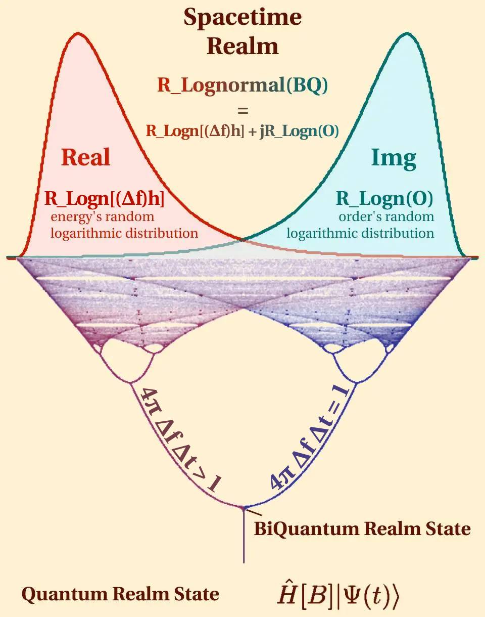
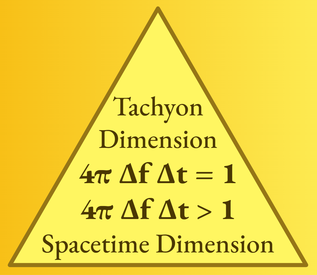
Asymmetric Bifurcation derived from the Quantum Energy randomness with BiQuantum Realm State, where Quantum Transform’s Bimodal Distribution is equal to the complex sum, the real part RLognormal[(Δf)h] is random logarithmic distribution representing changes in system’s frequency uncertainty, while the imaginary part RLognormal(O) is order’s random logarithmic distribution. 4π Δf Δt = N and 4π Δf Δt > 1 describe transition between the Minkowski space to tachyon space, where Δf is the frequency uncertainty and Δt is time uncertainty [4].
A quantum bifurcation oscillator model DAQ is a theoretical construct used in the field of quantum mechanics to describe the behavior of a quantum system that undergoes bifurcation. Bifurcation is a concept from nonlinear dynamics, and it occurs when a system transitions from one stable state to two or more distinct stable states as a parameter is varied. In the context of a quantum oscillator, this can involve the splitting of the quantum state into multiple branches, each corresponding to different stable states of the oscillator.
In classical mechanics, an oscillator follows a simple trajectory determined by its initial conditions and the equations of motion. However, in the quantum realm, the behavior of particles is described by wave functions and probabilistic outcomes. When a quantum oscillator undergoes bifurcation, the wave function may split into multiple branches, each representing a distinct stable state or trajectory.
Quantum bifurcation oscillators are often used as simplified models to study the quantum-to-classical transition and the emergence of classical behavior from quantum systems. Models DAQ can be used to explore the interplay between quantum coherence and classical chaos in complex systems.
The mathematical description of a quantum bifurcation oscillator typically involves nonlinear Schrödinger equation or some equivalent formalism, and it may incorporate the effects of external parameters that lead to bifurcation. These models can be quite challenging to analyze, and they are often used in theoretical studies and simulations to gain insight into the behavior of quantum systems in complex and nonlinear regimes.
Quantum Information Field Energy randomness observed at the multidimensional bifurcation point in spacetime can be described by Doktor Habdank’s formula
eq. 1, where H is the Hamiltonian at the multidimensional bifurcation point B, RLognormal(∆E) is a random log normal distribution of system’s energy changes, j is an imaginary number, φ(t) is a normal distribution expressed in Kelvins, and RLognormal(O) is a random log normal distribution of order (Longo 2009). This equation descrites a Hamiltonian operating at a certain point B, on a state |Ψ(t)⟩ which gives rise to a change in the system’s energy ∆E, which is distributed log-normally. This variability could be attributed to quantum fluctuations.
Eq.2 The plane wave solution to the Schrödinger equation for a free particle that is not subject to any potential energy, where: A is the amplitude of the wave, k is the wave number, ω is the angular frequency, x and t are the position and time variables, respectively, e is the base of the natural logarithm, and i is the imaginary unit.
Eq.3 Wave function is a two component object (ѱ1, ѱ2), which can be written as a complex number ѱ = ѱ1 + jѱ2, whose absolute square is |ѱ|2 = ѱ12 + ѱ22
Eq.4 An example of the Taylor series in quantum mechanics is the expansion of the time evolution operator, which is crucial for understanding how quantum states evolve over time. This series helps approximate the evolution of quantum states, especially for small t, and is foundational in developing more complex theories and techniques in quantum mechanics.
Eq.5 is time-frequency uncertainty relation derived from the more general Heisenberg Uncertainty Principle and eq.4 is a stricter form of the time-frequency uncertainty. The frequency uncertainty Δf, as described by the latter two equations, sets a limit on how accurately we can simultaneously know the frequency and duration of an event. Each equation describe one of the initial trajectories after BiQuantum Realm State point.
In quantum mechanics, energy and frequency are related by the Planck relation: E = h∗f, where E is energy, f is frequency, and ℎ is Planck’s constant.
Eq 8 is the probability of i-th element in all elements.
Eq 9 Nonlinear oscillator model, where:
R1, R2 ~ Random elements 1 and 2
C1, C2 ~ Capacitative elements 1 and 2
I ~ Field
U ~ Fields Potential
Eq 10 Generalized nonlinear oscillator model with 26 random (RN) and capacitative (CN) elements.
If there’s uncertainty in the energy ΔE, it will naturally induce an uncertainty in frequency Δf. This relation between energy and frequency, combined with the time-frequency uncertainty relations, suggests that when system’s energy changes are significant and fluctuate over a broad range (as indicated by a wide log-normal distribution), there’s a consequent broadening of the frequency uncertainty. These uncertainties in frequency, when combined with temporal uncertainties Δt, have to adhere to the constraints set by the time-frequency uncertainty relations provided.
The Quantum Model Learning Agent (QMLA) is an algorithm crafted to offer approximated, automated answers to the challenge of deducing a Hamiltonian model from empirical data. It proves useful especially when there’s prior knowledge of a parametrized Hamiltonian model [5].
Inputs that are maximally entangled contribute to tunnel tensor products, aiding in the examination of regularized versions of peak output orders, especially in context to the classical capacity challenge [6].
[3] Griffiths, David J. Introduction to Quantum Mechanics. 3rd ed., Cambridge University Press, 2018.
[4] Ross L. Dawe A and Kenneth C. Hines, “The Physics of Tachyons: I. Tachyon Kinematics, II. Tachyon Dynamics, III. Tachyon Electromagnetism“, Aust. J. Phys., 1992-1994, 45-47 (591-620, 725-38, 431-64)
[5] Antonio A. Gentile, et al., “Learning models of quantum systems from experiments“, Nature Physics, 2021
[6] Benoît Collins and Ion Nechita “Random matrix techniques in quantum information theory“, Journal of Mathematical Physics, 20120096